An overview of omics data

With a focus on high-throughput sequencing data

Jelmer Poelstra

August 26, 2026


The main omics data types

The main omics data types

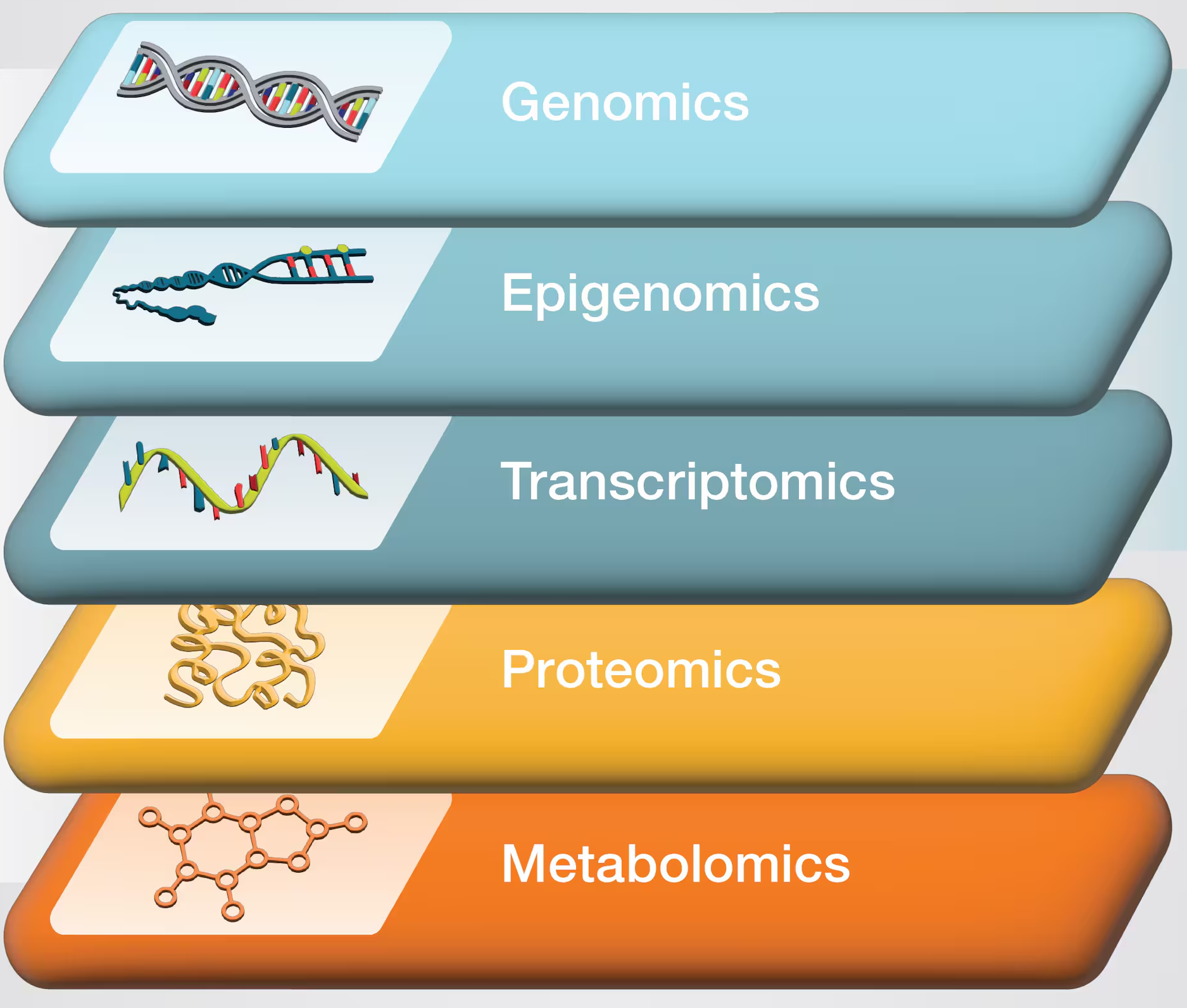
A diagram showing the main omics data types.

Copyright ThermoFisher

The main omics data types

Omics type Molecule type Shows
genomics DNA What can happen
epigenomics DNA modifications What is allowed to happen
transcriptomics RNA What appears to be targeted


What does -omics mean

The “omics” suffix indicates large-scale datasets — e.g., “genomics” data spans much or all of the genome.

While the boundaries can be fuzzy, sequencing a single gene is not genomics, and running qPCR for several genes is not transcriptomics.

The main omics data types

Omics type Molecule type Shows Mainly produced by
genomics DNA What can happen HTS
epigenomics DNA modifications What is allowed to happen HTS
transcriptomics RNA What appears to be targeted HTS


HTS = high-throughput sequencing

Nearly all HTS currently involves DNA sequencing, including for epigenomics and transcriptomics data. For example, RNA is reverse-transcribed prior to sequencing.

HTS is the focus of the rest of this lecture, and HTS data of examples throughout the course.

The main omics data types

Omics type Molecule type Shows Mainly produced by
genomics DNA What can happen HTS
epigenomics DNA modifications What is allowed to happen HTS
transcriptomics RNA What appears to be targeted HTS
proteomics proteins What is actively working
metabolomics metabolites What the net outcome is

The main omics data types

Omics type Molecule type Shows Mainly produced by
genomics DNA What can happen HTS
epigenomics DNA modifications What is allowed to happen HTS
transcriptomics RNA What appears to be targeted HTS
proteomics proteins What is actively working mass spectrometry
metabolomics metabolites What the net outcome is mass spectrometry


Multi-omics

In multi-omics studies, two or more omics data types are combined — ideally from the same set of samples.

This is often needed to link genotype to phenotype. For example, to study a plant-pathogen interaction, one could combine host and pathogen transcriptomics with metabolomics of plant defense compounds.

Learn more in this week’s first reading

Poinsignon et al. (2023) — Working with omics data:
An interdisciplinary challenge at the crossroads of biology and computer science


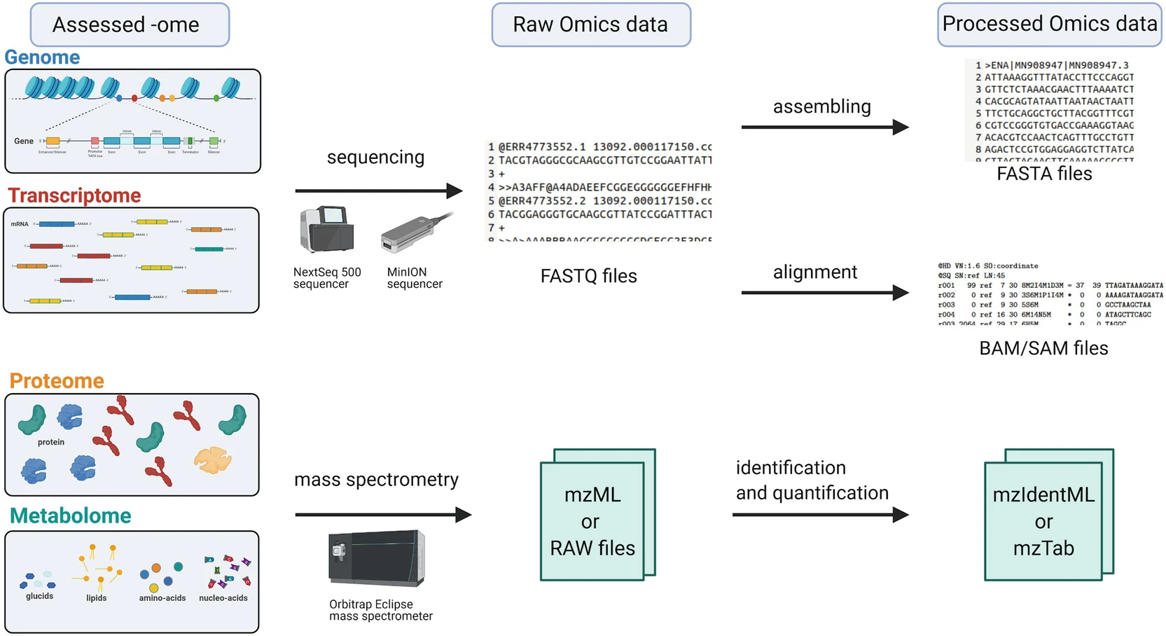
A diagram showing how different kinds of omics data are produced and analyzed.

Figure 2 from the paper.

High-throughput sequencing (HTS)

Sanger vs. high-throughput sequencing

Sanger sequencing

  • Since 1977 (technology) / 1986 (automated sequencer).

  • Sequencing of a single, short-ish DNA fragment at a time.

  • This fragment is typically PCR-amplified and therefore specifically targeted.

High-throughput sequencing (HTS)

  • Since 2005.
    x

  • Sequencing of hundreds of thousands to billions of DNA fragments at a time.

  • Fragments can be targeted in various ways or randomly generated from input DNA.


Reads and sequencing errors

The sequence determined from a DNA fragment is called a “read”. With current technologies, reads are never 100% accurate, and this has important consequences for downstream analyses.

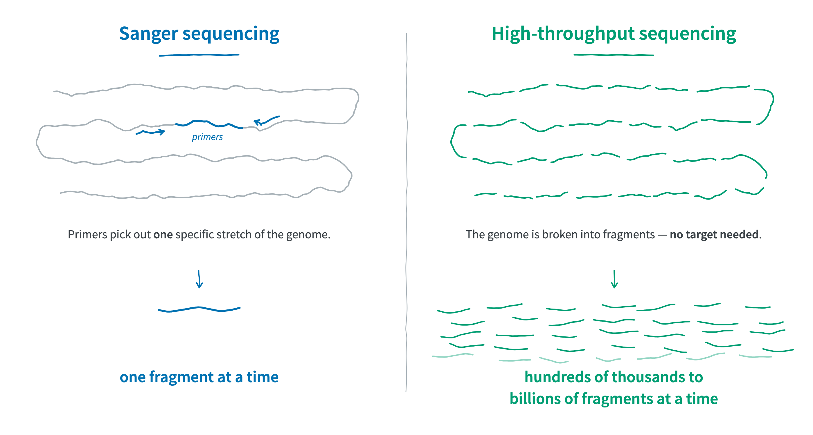
Two panels comparing what is sequenced. Left, Sanger sequencing: a folded, squiggly genome drawn in grey with one short stretch highlighted in blue, flanked by two primers pointing inwards; below it, a single blue fragment, labelled one fragment at a time. Right, high-throughput sequencing: the same squiggly genome, now broken into many teal fragments; below it, a large pile of teal fragments, labelled hundreds of thousands to billions of fragments at a time.

Timeline

First automated Sanger sequencer

First high-throughput sequencer, by 454

First Illumina sequencer

First long-read sequencer, by PacBio

First Oxford Nanopore sequencer,
the pocket-sized MinION


Do you know when first the human genome assembly was published? The first draft of the human genome was published in 2001.

The main HTS technologies

Short-read HTS Long-read HTS
Main technologies Illumina Oxford Nanopore Technologies (ONT) & Pacific Biosciences (PacBio)

The main HTS technologies

Short-read HTS Long-read HTS
Usage most common less common (but increasing)
Main technologies Illumina Oxford Nanopore Technologies (ONT) & Pacific Biosciences (PacBio)
Timeline since 2006 — technology fairly stable since 2011 — still rapid development

The main HTS technologies

Short-read HTS Long-read HTS
Usage most common less common (but increasing)
Main technologies Illumina Oxford Nanopore Technologies (ONT) & Pacific Biosciences (PacBio)
Timeline since 2006 — technology fairly stable since 2011 — still rapid development
Read lengths 50–300 bp 10–100+ kbp
Error rates mostly <0.1% 0.5–1% (ONT) / mostly <0.1% (PacBio)

Long reads are orders of magnitude longer than short reads — and, for PacBio, just as accurate.

So why is Illumina still by far the most commonly used HTS technology?

The main HTS technologies

Short-read HTS Long-read HTS
Usage most common less common (but increasing)
Main technologies Illumina Oxford Nanopore Technologies (ONT) & Pacific Biosciences (PacBio)
Timeline since 2006 — technology fairly stable since 2011 — still rapid development
Read lengths 50–300 bp 10–100+ kbp
Error rates mostly <0.1% 0.5–1% (ONT) / mostly <0.1% (PacBio)
Throughput higher lower
Cost per base lower higher

The main HTS technologies

Short-read HTS Long-read HTS
Usage most common less common (but increasing)
Main technologies Illumina Oxford Nanopore Technologies (ONT) &
Pacific Biosciences (PacBio)
Timeline since 2006 — technology fairly stable since 2011 — still rapid development
Read lengths 50–300 bp 10–100+ kbp
Error rates mostly <0.1% 0.5–1% (ONT) / mostly <0.1% (PacBio)
Throughput higher lower
Cost per base lower higher
AKA Next-Generation Sequencing (NGS) Third-Generation Sequencing (TGS)

Examples of HTS applications

  • Genome assembly

  • Variant analysis — for population genetics/genomics, GWAS, etc.

  • Gene expression comparisons — using RNA-Seq

  • Microbial community characterization — using metabarcoding or shotgun metagenomics


For which of these applications are longer reads very useful?
  • Genome assembly
  • Microbial community characterization
For which of these applications is read length not as important?
  • Variant analysis
  • Gene expression comparisons — and many other “read-as-a-tag” applications where the goal is just to know a read’s origin in a reference genome.
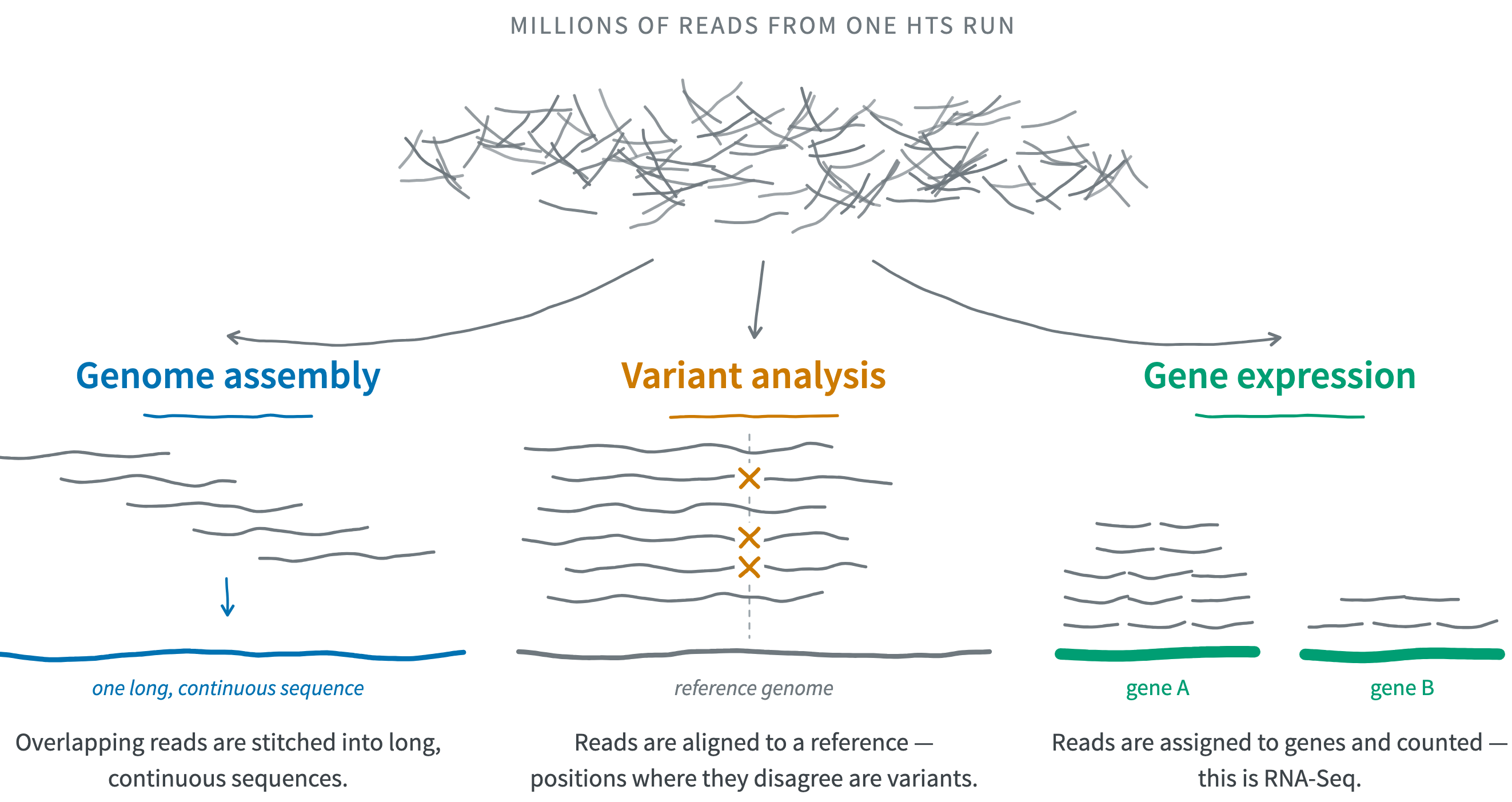
Three HTS applications sketched from one starting point. At the top, a dense, unstructured pile of short reads labelled millions of reads from one HTS run, with three arrows fanning down. Left, genome assembly: five reads arranged as a staircase so each overlaps the one above, an arrow, and a single long blue line labelled one long, continuous sequence. Middle, variant analysis: six reads aligned above a grey reference genome line, with an amber cross at the same column in three of the six. Right, gene expression: reads sorted into two stacks, a tall stack over a teal bar labelled gene A and a short stack over a bar labelled gene B.

The two stages of many HTS analyses

Algorithmic initial data processing

Typically:

  • Operates on reads, alignments, and so on.
  • Done in a Unix shell on a supercomputer.
  • Relatively standardized, automatable, and “non-interactive”.

Statistical analysis & visualization

Typically:

  • Operates on summaries like read counts.
  • Can be done with R on a laptop.
  • Highly interactive and iterative, less standardized and harder to automate.

Examples:

  • Read quality control (QC) and trimming.
  • Alignment of reads to a reference genome.
  • Comparing counts of genes (RNA-Seq) or taxa (metabarcoding) among treatments.
  • Genome-wide Association Studies (GWAS).

HTS recap

HTS & Omics

HTS produces the most common omics data types:

  • genomics
  • transcriptomics
  • (and epigenomics)

Read types

Three technologies are most commonly used, producing reads that are:

  • short (Illumina) or
  • long (ONT and PacBio)

Applications

Many applications exist.

Some are not (just) about determining the exact DNA sequence, but about producing counts of categories like genes.

Illumina libraries and sequencing

Illumina libraries and sequencing

We’re going to zoom in on Illumina sequencing, because:

  • This is the most commonly used type of HTS.
  • We’ll use Illumina read files as examples throughout the course.

%%{init: {'themeCSS': '.edgePath .path, .flowchart-link { stroke-width: 3px; }'}}%%
flowchart TD
    Omics([Omics technologies])
    HTS[HTS]
    MS[Mass spectrometry]
    Illumina[Illumina]
    ONT[ONT]
    PacBio[PacBio]

    Omics --> HTS
    Omics --> MS
    HTS --> Illumina
    HTS --> ONT
    HTS --> PacBio

    classDef omics fill:#bb0000,color:#ffffff,stroke:#bb0000,font-weight:bold;
    classDef hts fill:#009E73,color:#ffffff,stroke:#009E73,font-weight:bold;
    classDef illumina fill:#0072B2,color:#ffffff,stroke:#0072B2,font-weight:bold;
    classDef dim fill:#eaeaea,color:#999999,stroke:#cccccc;

    class Omics omics;
    class HTS hts;
    class Illumina illumina;
    class MS,ONT,PacBio dim;


Libraries and library prep

In a sequencing context, a “library” is a collection of
nucleic acid fragments ready for sequencing.


These fragments number in the millions or billions and are
often simply generated at random from input such as genomic DNA:

A diagram showing the main Illumina library preparation steps.

An overview of the library prep procedure. This is typically done for you by a sequencing facility or company.

A closer look at the processed DNA fragments

As shown on the previous slide, after library prep,
each DNA fragment is flanked by several types of short sequences
that together make up the “adapters”:


A diagram of a DNA fragment in a prepared library, with adapters flanking the fragment.


Multiplexing!

Adapters can include so-called “indices” or “barcodes” that identify individual samples.
That way, many samples can be combined (multiplexed) into a single library.

Paired-end vs. single-end sequencing

DNA fragments can be sequenced from both ends as shown below,
and this is called “paired-end” (PE) sequencing:

A diagram showing forward and reverse reads in paired-end sequencing.


Why paired-end sequencing?

This is a way for Illumina sequencing to produce more information from the same DNA fragment, given the limited read length of the technology (as you always know which two reads form a pair).

Paired-end vs. single-end sequencing

DNA fragments can be sequenced from both ends as shown below,
and this is called “paired-end” (PE) sequencing:

A diagram showing forward and reverse reads in paired-end sequencing.


When sequencing is instead single-end (SE), no reverse read is produced:

A diagram showing the forward read in single-end sequencing.

Insert size variation

The DNA fragment’s size (“insert size”) can vary — by design, but also
because of limited precision in size selection. What happens when it is:


1: Shorter than the combined read length (but longer than a single read)?

  1. The fragment is too short to sequence, so it drops out of the library.
  2. The forward and reverse reads overlap in the middle.
  3. The reads come out shorter than the read length that was ordered.
  4. The final bases of each read consist of adapter sequence.

A diagram illustrating the scenario when the DNA fragment is shorter than the combined read length

Insert size variation

The DNA fragment’s size (“insert size”) can vary — by design, but also
because of limited precision in size selection. What happens when it is:


2: Shorter than a single read? (The reads still overlap — but what else?)

  1. The sequencer stops early, so these reads are shorter than the rest.
  2. The reverse read is dropped, leaving only a forward read.
  3. The final bases of each read consist of adapter sequence.
  4. The fragment gets sequenced twice, producing a PCR duplicate.
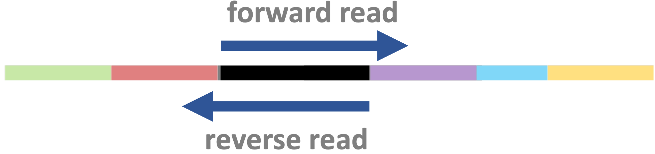
A diagram illustrating the scenario when the DNA fragment is shorter than the single read length

Video of Illumina technology

Reference genomes

Reference genomes

Many HTS applications require a “reference genome” (or involve its production), which includes:

An assembly

The assembled genomic DNA sequence, in pieces ranging up to whole chromosomes.

  • Most genome assemblies are incomplete and fragmented (but less and less so).

  • Non-chromosome-level pieces are called contigs and scaffolds.

An annotation

Provides the locations of genes and other genomic “features”, plus functional information about them.

Reference genomes are typically applicable at the species level. But:

  • If needed, it’s often possible to work with genomes of closely related species.
  • Conversely, different subspecies/lines may have their own reference genomes.

Illumina and reference genome recap

Library prep

Prepares nucleic acid fragments for sequencing.

For example, by attaching adapter and sample barcode sequences.

Sequencing design

Illumina sequencing is often done with:

  • Paired-end reads
  • Multiple samples at a time (multiplexing)

Reference genome

For many omics analyses, you need a reference genome assembly and annotation.

The course’s main example dataset

Garrigós et al. 2025

Throughout the course, we’ll use an example/practice data set from Garrigós et al. (2025):
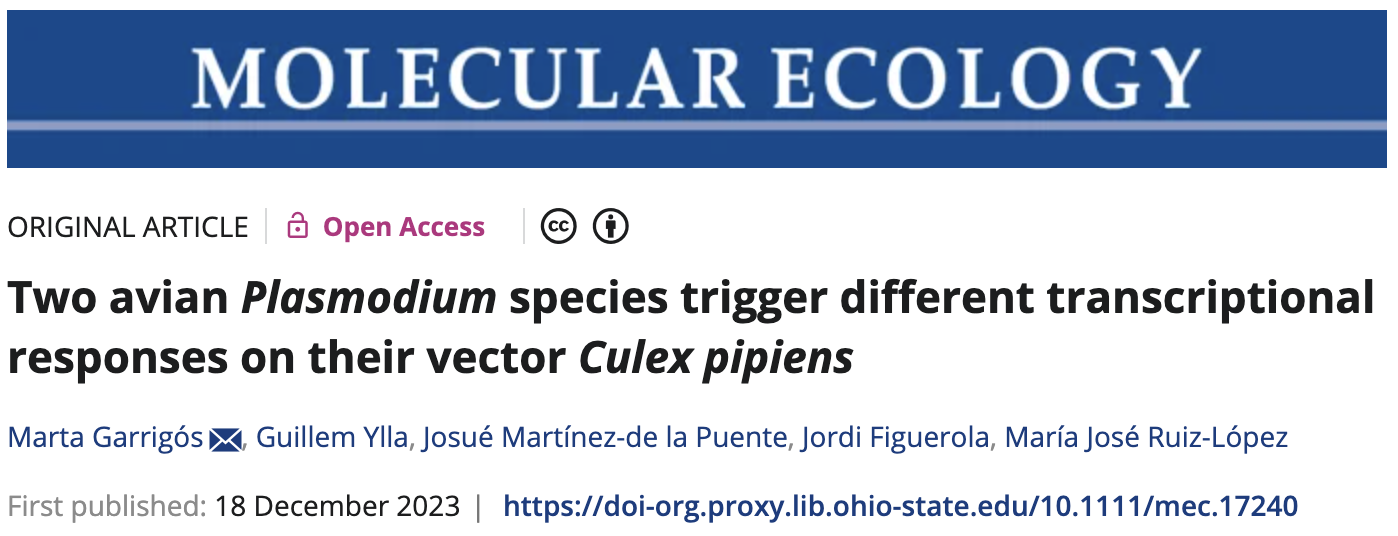
A screenshot of the paper's front matter.

This paper uses paired-end Illumina RNA-Seq data to study gene expression in Culex pipiens mosquitoes infected with two different malaria-causing Plasmodium protozoans.

What’s next?

At the start of week 4, we’ll discuss follow-up material related to today’s lecture:

  • Sequence file types, such as FASTQ files that contain the reads produced by HTS.

  • More on the Garrigós et al. (2025) dataset (the paper is that week’s assigned reading).

  • An overview of the RNA-Seq data analysis steps we’ll perform on the Garrigós dataset.

Questions?


Break for 5 minutes

References

Garrigós, Marta, Guillem Ylla, Josué Martínez-de la Puente, Jordi Figuerola, and María José Ruiz-López. 2025. “Two Avian Plasmodium Species Trigger Different Transcriptional Responses on Their Vector Culex pipiens.” Molecular Ecology 34 (15): e17240. https://doi.org/10.1111/mec.17240.
Poinsignon, Thibault, Pierre Poulain, Mélina Gallopin, and Gaëlle Lelandais. 2023. Working with Omics Data: An Interdisciplinary Challenge at the Crossroads of Biology and Computer Science. Humana, New York, NY. https://doi.org/10.1007/978-1-0716-3195-9_10.